RoboticsAcademy Challenge#
This is my solution to the RoboticsAcademy Challenge
Visual Follow Line#
This exercise requires a PID controller to drive an F1 car in race circuit. This has 2 parts:
Approach#
Computer Vision#
This part focuses on using OpenCv library to detect the red line in the circuit so that the controller can take actions nased on it.
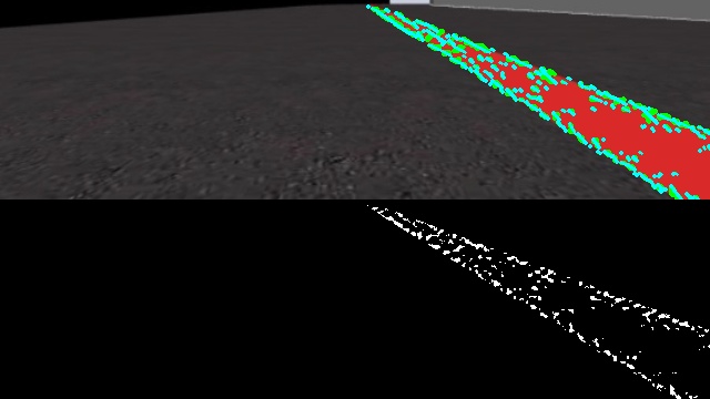
I have used filtering in HSV space based on the if pixel value is between the given threshold. I have used two HSV thresholds for red colour to create a mask in the region of interest
These are outputs using indivdual thresholds
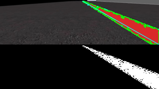
Now, using both the masks together we get a better result
51mask1 = cv2.inRange(hsv, lower_red1, upper_red1)
52mask2 = cv2.inRange(hsv, lower_red2, upper_red2)
53mask = mask1 | mask2

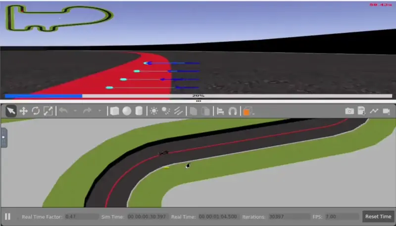
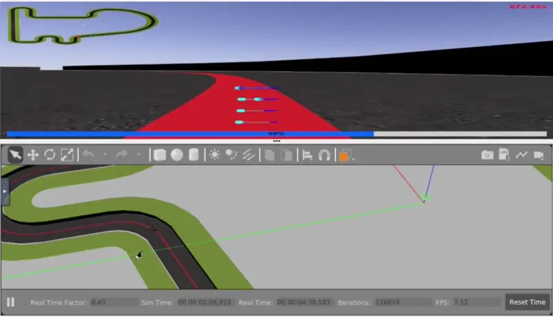
Next, I have used multiple ROIs instead of one, because of the curved nature of the path. For each ROIs I have found the moment and it’s distance from the center. The deviation from centre is then calculated by taking the average of these distances.
However, not all distances are weighted equally. The ROI in the centre has the maximum weightage, then it neighbours above and below, and so on. This way the ROI very close to the wheel and farthest from the wheel have less weightage.
To achive this I have used the following function
def create_symmetric_array(length):
    middle = length // 2
    half = np.arange(1, middle + 1, dtype=float)  # Create an array [1, 2, ..., middle] with float dtype
    arr = np.concatenate((half, [] if length % 2 == 0 else [middle + 1], half[::-1]))  # Concatenate arrays to form the symmetric array
    arr /= np.linalg.norm(arr, ord=1)  # Normalize the array so that the sum of its elements is 1
    return arr
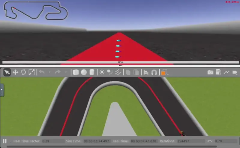
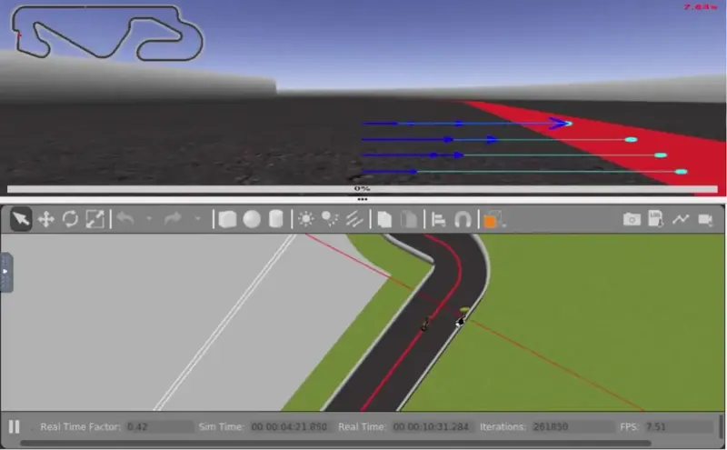
The result looks this this:
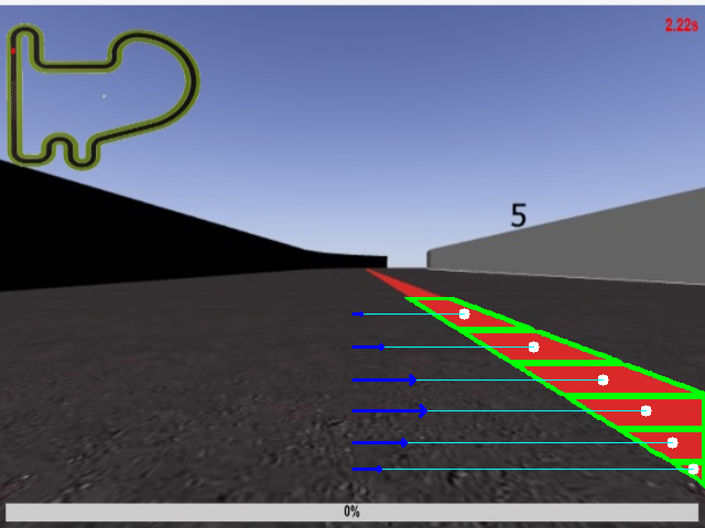
Enclosed in Green border shows different ROIs, where the white circle is their moments. Cyan colored Line shows the distance from the center and the Blue arrows represent the weightage of these distances.#
Control System#
PID controller has been used to make the car follow the line. The distance from the centre is takes as an error and used in feedback loop for the angular and linear velocity. The angular velocity uses PID while the linear velocity just uses differential controller. The reason being that the car will run a a fixed speed and slow down near turns.
Ziegler–Nichols#
I have used the Ziegler–Nichols method for tuning this PID controller.
The “P” (proportional) gain, \(K_{p}\) is then increased (from zero) until it reaches the ultimate gain \(K_{u}\), at which the output of the control loop has stable and consistent oscillations.
–Wikipedia (Ziegler–Nichols method)
So I increased my \(K_{p}\) value from \(0.001\) to \(0.02\). The best performance I saw was at \(K_{p} = 0.005\) and we will see that Ziegler–Nichols method will also give the same conclusion.
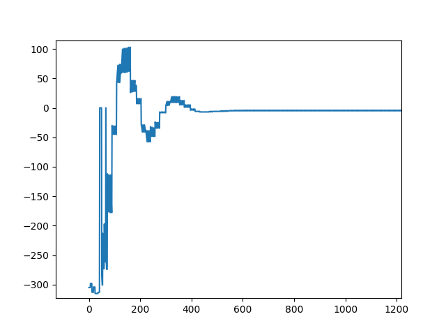
At \(K_{p} = 0.02\) we have unstable oscillations that break the system. Notice the car complete deviates from the centre at the end of the movie.
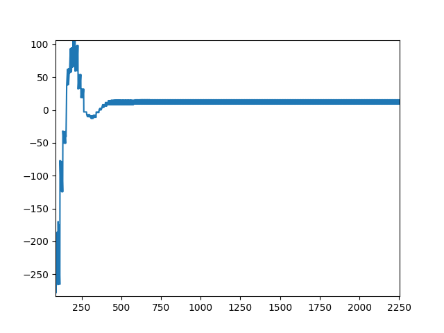
Here are the stable and consistent oscillations giving the value \(K_{u} = 0.015\)
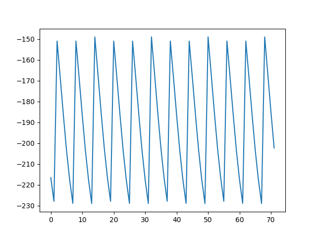
Error plot for \(K_{p} = 0.015\) showing stable and consistent oscillations.#
Now, with time period \(T_{u} = 6 \times 20\), the values of \(K_p\), \(K_i\) and \(K_d\) are found to be
Control Type |
\(K_{p}\) |
\(K_{i}\) |
\(K_{d}\) |
|---|---|---|---|
some overshoot |
\(0.0049\bar{9}\) |
\(0.000083\bar{3}\) |
\(0.19\bar{9}\) |
I have not used these crude values directly, but tune a bit more from this point where \(K_{d}\) was changed to \(0.002\)
PID Test#
After finalizing the propotional, integral and differential constants, the out put of system on disturbance was tested and gave satisfactory results.
Simulation#
For entire simuation watch the YouTube videos.
Here are few clips showing the performance of the PID path following F1 car.
Simple World#
1. 90° Corner turn#
90° Corner turn of Simple World#
2. Hairpin Turn#
Hairpin turn of Simple World#
Montmeló World#
1. La Caixa (sharp 135° left)#
La Caixa, sharp 135° left turn of Montmelo World#
2. [Crash] Europcar (sharp 75° right)#

Europcar corner, sharp 75° right turn of Montmelo World#
3. [Crash] Chicane#
Left-Right Chicane of Montmelo World#
Source Code#
PID_controller.py
The source code is available on github but has been encrypted. To view the code follow these commands
wget https://raw.githubusercontent.com/ABD-01/crispy-adventure/master/RoboticsAcademy/PID_controller.py.data
openssl enc -aes-128-cbc -d -a -pbkdf2 -in PID_controller.py.data -out PID_controller.py
The key to decrypt the file has been provided in the email.
Use of AI and Symmetric Arrays#
Why add this section? Because I read a discussion where … (you have read that part already. If not see Python or ROS2)
Honesty requires me to mention that I have used assitance of ChatGPT for create_symmetric_array
Symmetric Arrays
Although that is not what I intended. I wanted to weight the distances such that the weights form a normal distribution. Something like this:
num = 50
weights = norm.pdf(np.arange(num), num // 2, num//4)
plt.bar(np.arange(num) , weights)
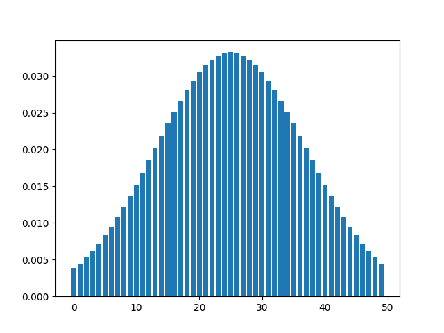
.png)
But what I got and moved forward with is this:
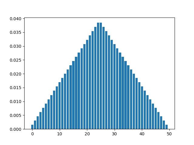
.png)
References#
Multiple Thresholds for Red: OpenCV better detection of red color?
HSV Ranges: Identifying the range of a color in HSV using OpenCV
Centre of a ROI: Find the Center of a Blob (Centroid) using OpenCV (C++/Python)
Creating symmetric arrays How to generate a random normal distribution of integers
PID Tuning: Ziegler–Nichols method